
Overview
SQL (Structured Query Language) is a standard language for data operations that allows you to ask questions and get insights from structured datasets. It's commonly used in database management and allows you to perform tasks like transaction record writing into relational databases and petabyte-scale data analysis.
This lab serves as an introduction to SQL and is intended to prepare you for the many labs and quests in Qwiklabs on data science topics. This lab is divided into two parts: in the first half, you will learn fundamental SQL querying keywords, which you will run in the BigQuery console on a public dataset that contains information on London bikeshares.
In the second half, you will learn how to export subsets of the London bikeshare dataset into CSV files, which you will then upload to Cloud SQL. From there you will learn how to use Cloud SQL to create and manage databases and tables. Towards the end, you will get hands-on practice with additional SQL keywords that manipulate and edit data.
Objectives
In this lab, you will learn how to:
Distinguish databases from tables and projects.
Use the SELECT, FROM, and WHERE keywords to construct simple queries.
Identify the different components and hierarchies within the BigQuery console.
Load databases and tables into BigQuery.
Execute simple queries on tables.
Learn about the COUNT, GROUP BY, AS, and ORDER BY keywords.
Execute and chain the above commands to pull meaningful data from datasets.
Export a subset of data into a CSV file and store that file into a new Cloud Storage bucket.
Create a new Cloud SQL instance and load your exported CSV file as a new table.
Run CREATE DATABASE, CREATE TABLE, DELETE, INSERT INTO, and UNION queries in Cloud SQL.
Prerequisites
Very Important: Before starting this lab, log out of your personal or corporate gmail account.
This is a introductory level lab. This assumes little to no prior experience with SQL. Familiarity with Cloud Storage and Cloud Shell is recommended, but not required. This lab will teach you the basics of reading and writing queries in SQL, which you will apply by using BigQuery and Cloud SQL.
Source:
This lab is from Qwiklabs.
Task 1: Sign in to the Google Cloud Platform (GCP) Console

The Basics of SQL
Databases and Tables
As mentioned earlier, SQL allows you to get information from "structured datasets". Structured datasets have clear rules and formatting and often times are organized into tables, or data that's formatted in rows and columns.
An example of unstructured data would be an image file. Unstructured data is inoperable with SQL and cannot be stored in BigQuery datasets or tables (at least natively.) To work with image data (for instance), you would use a service like Cloud Vision, perhaps through its API directly.
The following is an example of a structured dataset—a simple table:

If you've had experience with Google Sheets, then the above should look quite similar. As we see, the table has columns for User, Price, and Shipped and two rows that are composed of filled in column values.
A Database is essentially a collection of one or more tables. SQL is a structured database management tool, but quite often (and in this lab) you will be running queries on one or a few tables joined together—not on whole databases.
SELECT and FROM
SQL is phonetic by nature and before running a query, it's always helpful to first figure out what question you want to ask your data (unless you're just exploring for fun.)
SQL has predefined keywords which you use to translate your question into the pseudo-english SQL syntax so you can get the database engine to return the answer you want.
The most essential keywords are SELECT and FROM:
Use SELECT to specify what fields you want to pull from your dataset.
Use FROM to specify what table or tables we want to pull our data from.
An example may help understanding. Assume that we have the following table example_table, which has columns USER, PRICE, and SHIPPED:

And let's say that we want to just pull the data that's found in the USER column. We can do this by running the following query that uses SELECT and FROM:
SELECT USER FROM example_table
If we executed the above command, we would select all the names from the USER column that are found in example_table.
You can also select multiple columns with the SQL SELECT keyword. Say that you want to pull the data that's found in the USER and SHIPPED columns. To do this, modify the previous query by adding another column value to our SELECT query (making sure it's separated by a comma!):
SELECT USER, SHIPPED FROM example_table
Running the above retrieves the USER and the SHIPPED data from memory:

And just like that you've covered two fundamental SQL keywords! Now to make things a bit more interesting.
WHERE
The WHERE keyword is another SQL command that filters tables for specific column values. Say that you want to pull the names from example_table whose packages were shipped. You can supplement the query with a WHERE, like the following:
SELECT USER FROM example_table WHERE SHIPPED='YES'
Running the above returns all USERs whose packages have been SHIPPED from memory:

Now that you have a baseline understanding of SQL's core keywords, apply what you've learned by running these types of queries in the BigQuery console.
Exploring the BigQuery Console
The BigQuery paradigm
BigQuery is a fully-managed petabyte-scale data warehouse that runs on the Google Cloud. Data analysts and data scientists can quickly query and filter large datasets, aggregate results, and perform complex operations without having to worry about setting up and managing servers. It comes in the form of a command line tool (preinstalled in cloudshell) or a web console—both ready for managing and querying data housed in Google Cloud projects.
In this lab, you use the web console to run SQL queries.
Open BigQuery Console
In the Google Cloud Console, select Navigation menu > BigQuery:

The Welcome to BigQuery in the Cloud Console message box opens. This message box provides a link to the quickstart guide and the release notes.
Click Done.
The BigQuery console opens.

Take a moment to note some important features of the UI. The right-hand side of the console houses the query "Editor". This is where you write and run SQL commands like the examples we covered earlier. Below that is "Query history", which is a list of queries you ran previously.
The left pane of the console is the "Navigation panel". Apart from the self-explanatory query history, saved queries, and job history, there is the Explorer tab.
The highest level of resources in Explorer tab contain Google Cloud projects, which are just like the temporary Google Cloud projects you sign in to and use with each Qwiklab. As you can see in your console and in the last screenshot, we only have our Qwiklabs project housed in the Explorer tab. If you try clicking on the arrow next the project name, nothing will show up.
This is because your project doesn't contain any datasets or tables, you have nothing that can be queried. Earlier you learned datasets contain tables. When you add data to your project, note that in BigQuery, projects contain datasets, and datasets contain tables. Now that you better understand the project → dataset → table paradigm and the intricacies of the console, you can load up some queryable data.
Uploading queryable data
In this section you pull in some public data into your project so you can practice running SQL commands in BigQuery.
Click on the + ADD DATA link then select Explore public datasets:

In the search bar, enter "london" and press Enter, then select the London Bicycle Hires tile, then View Dataset.
A new tab will open, and you will now have a new project called bigquery-public-data added to the Explorer panel:

It's important to note that you are still working out of your lab project in this new tab. All you did was pull a publicly accessible project that contains datasets and tables into BigQuery for analysis — you didn't switch over to that project. All of your jobs and services are still tied to your Qwiklabs account. You can see this for yourself by inspecting the project field near the top of the console:

Expand bigquery-public-data > london_bicycles and select cycle_hire. You now have data that follows the BigQuery paradigm:
Google Cloud Project → bigquery-public-data
Dataset → london_bicycles
Table → cycle_hire
Now that you are in the cycle_hire table, in the center of the console click the Preview tab. Your page should resemble the following:

Inspect the columns and values populated in the rows. You are now ready to run some SQL queries on the cycle_hire table.
Running SELECT, FROM, and WHERE in BigQuery
You now have a basic understanding of SQL querying keywords and the BigQuery data paradigm and some data to work with. Run some SQL commands using this service.
If you look at the bottom right corner of the console, you will notice that there are 24,369,201 rows of data, or individual bikeshare trips taken in London between 2015 and 2017 (not a small amount by any means!)
Now take note of the seventh column key: end_station_name, which specifies the end destination of bikeshare rides. Before we get too deep, let's first run a simple query to isolate the end_station_name column. Copy and paste the following command in to the query EDITOR:
SELECT end_station_name FROM `bigquery-public-data.london_bicycles.cycle_hire`;
Then click Run.
After ~20 seconds, you should be returned with 24369201 rows that contain the single column you queried for: end_station_name.
Why don't you find out how many bike trips were 20 minutes or longer?
Clear the query from the editor, then run the following query that utilizes the WHERE keyword:
SELECT * FROM `bigquery-public-data.london_bicycles.cycle_hire` WHERE duration>=1200;
This query may take a minute or so to run.
SELECT * returns all column values from the table. Duration is measured in seconds, which is why you used the value 1200 (60 * 20).
If you look in the bottom right corner you see that 7,334,890 rows were returned. As a fraction of the total (7334890/24369201), this means that ~30% of London bikeshare rides lasted 20 minutes or longer (they're in it for the long haul!)

More SQL Keywords: GROUP BY, COUNT, AS, and ORDER BY
GROUP BY
The GROUP BY keyword will aggregate result-set rows that share common criteria (e.g. a column value) and will return all of the unique entries found for such criteria.
This is a useful keyword for figuring out categorical information on tables. To get a better picture of what this keyword does, clear the query from the editor, then copy and paste the following command:
SELECT start_station_name FROM `bigquery-public-data.london_bicycles.cycle_hire` GROUP BY start_station_name;
Click Run.
You should receive a similar output (row values may not match the following):

Without the GROUP BY, the query would have returned the full 24,369,201 rows. GROUP BY will output the unique (non-duplicate) column values found in the table. You can see this for yourself by looking in the bottom right corner. You will see 880 rows, meaning there are 880 distinct London bikeshare starting points.
COUNT
The COUNT() function will return the number of rows that share the same criteria (e.g. column value). This can be very useful in tandem with a GROUP BY.
Add the COUNT function to our previous query to figure out how many rides begin in each starting point. Clear the query from the editor, then copy and paste the following command and then click Run:
SELECT start_station_name, COUNT(*) FROM `bigquery-public-data.london_bicycles.cycle_hire` GROUP BY start_station_name;
You should receive a similar output (row values may not match the following):

This shows how many bikeshare rides begin at each starting location.
AS
SQL also has an AS keyword, which creates an alias of a table or column. An alias is a new name that's given to the returned column or table—whatever AS specifies.
Add an AS keyword to the last query we ran to see this in action. Clear the query from the editor, then copy and paste the following command:
SELECT start_station_name, COUNT(*) AS num_starts FROM `bigquery-public-data.london_bicycles.cycle_hire` GROUP BY start_station_name;
Click Run.
You should receive a similar output (be aware that the row values might not be identical):

As you see, the COUNT(*) column in the returned table is now set to the alias name num_starts. This is a handy keyword to use especially if you are dealing with large sets of data — forgetting that an ambiguous table or column name happens more often than you think!
ORDER BY
The ORDER BY keyword sorts the returned data from a query in ascending or descending order based on a specified criteria or column value. We will add this keyword to our previous query to do the following:
Return a table that contains the number of bikeshare rides that begin in each starting station, organized alphabetically by the starting station.
Return a table that contains the number of bikeshare rides that begin in each starting station, organized numerically from lowest to highest.
Return a table that contains the number of bikeshare rides that begin in each starting station, organized numerically from highest to lowest.
Each of the commands below is a separate query. For each command, clear the query EDITOR, copy and paste the command in to the query EDITOR, and then click Run. Examine the results.
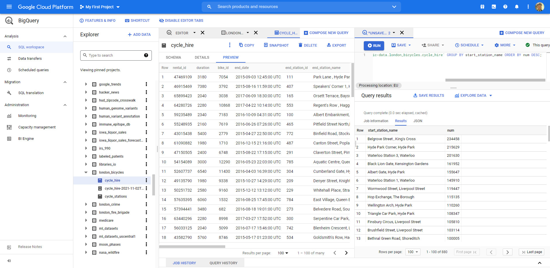
SELECT start_station_name, COUNT(*) AS num FROM `bigquery-public-data.london_bicycles.cycle_hire` GROUP BY start_station_name ORDER BY start_station_name;

SELECT start_station_name, COUNT(*) AS num FROM `bigquery-public-data.london_bicycles.cycle_hire` GROUP BY start_station_name ORDER BY num;

SELECT start_station_name, COUNT(*) AS num FROM `bigquery-public-data.london_bicycles.cycle_hire` GROUP BY start_station_name ORDER BY num DESC;

We see that "Belgrove Street, King's Cross" has the highest number of starts. However, as a fraction of the total (234458/24369201), we see that < 1% of rides start from this station.
Working with Cloud SQL
Exporting queries as CSV files
Cloud SQL is a fully-managed database service that makes it easy to set up, maintain, manage, and administer your relational PostgreSQL and MySQL databases in the cloud. There are two formats of data accepted by Cloud SQL: dump files (.sql) or CSV files (.csv). You will learn how to export subsets of the cycle_hire table into CSV files and upload them to Cloud Storage as an intermediate location.
Back in the BigQuery Console, this should have been the last command that you ran:
SELECT start_station_name, COUNT(*) AS num FROM `bigquery-public-data.london_bicycles.cycle_hire` GROUP BY start_station_name ORDER BY num DESC;
In the Query Results section click SAVE RESULTS > CSV(local file) > SAVE. This initiates a download, which saves this query as a CSV file. Note the location and the name of this downloaded file—you will need it soon.
Clear the query EDITOR, then copy and run the following in the query editor:
SELECT end_station_name, COUNT(*) AS num FROM `bigquery-public-data.london_bicycles.cycle_hire` GROUP BY end_station_name ORDER BY num DESC;
This will return a table that contains the number of bikeshare rides that finish in each ending station and is organized numerically from highest to lowest number of rides. You should receive the following output:

In the Query Results section click SAVE RESULTS > CSV(local file) > SAVE. This initiates a download, which saves this query as a CSV file. Note the location and the name of this downloaded file—you will need it in the following section.
Upload CSV files to Cloud Storage
Go to the Cloud Console where you'll create a storage bucket where you can upload the files you just created.
Select Navigation menu > Cloud Storage > Browser, and then click CREATE BUCKET.
Note: If prompted, Click LEAVE for Unsaved work.
Enter a unique name for your bucket, keep all other settings as default, and click Create:

Create a cloud storage bucket.
You should now be in the Cloud Console looking at your newly created Cloud Storage Bucket.
Click UPLOAD FILES and select the CSV that contains start_station_name data. Then click Open. Repeat this for the end_station_name data.
Rename your start_station_name file by clicking on the three dots next to on the far side of the file and click rename. Rename the file to start_station_data.csv.
Rename your end_station_name file by clicking on the three dots next to on the far side of the file and click rename. Rename the file to end_station_data.csv.
Your bucket should now resemble the following:

Create a Cloud SQL instance
In the console, select Navigation menu > SQL.
Click CREATE INSTANCE.
From here, you will be prompted to choose a database engine. Select MySQL.
Now enter in a name for your instance (like "qwiklabs-demo") and enter a secure password in the Password field (remember it!), then click CREATE INSTANCE:

It might take a few minutes for the instance to be created. Once it is, you will see a green checkmark next to the instance name.
Click on the Cloud SQL instance. You should now be on a page that resembles the following:

New Queries in Cloud SQL
CREATE keyword (databases and tables)
Now that you have a Cloud SQL instance up and running, create a database inside of it using the Cloud Shell Command Line.
Activate Cloud Shell
Cloud Shell is a virtual machine that is loaded with development tools. It offers a persistent 5GB home directory and runs on the Google Cloud. Cloud Shell provides command-line access to your Google Cloud resources.
In the Cloud Console, in the top right toolbar, click the Activate Cloud Shell button.
Click Continue.
It takes a few moments to provision and connect to the environment. When you are connected, you are already authenticated, and the project is set to your PROJECT_ID. For example:
Run the following command in Cloud Shell to connect to your SQL instance, replacing qwiklabs-demo if you used a different name for your instance:
gcloud sql connect qwiklabs-demo --user=root
It may take a minute to connect to your instance.
When prompted, enter the root password you set for the instance.
You should now be on a similar output:

A Cloud SQL instance comes with pre-configured databases, but you will create your own to store the London bikeshare data.
Run the following command at the MySQL server prompt to create a database called bike:
CREATE DATABASE bike;
You should receive the following output:
Query OK, 1 row affected (0.05 sec)mysql>
Make a table inside of the bike database by running the following command:
USE bike;CREATE TABLE london1 (start_station_name VARCHAR(255), num INT);
This statement uses the CREATE keyword, but this time it uses the TABLE clause to specify that it wants to build a table instead of a database. The USE keyword specifies a database that you want to connect to. You now have a table named "london1" that contains two columns, "start_station_name" and "num". VARCHAR(255) specifies variable length string column that can hold up to 255 characters and INT is a column of type integer.
Create another table named "london2" by running the following command:
USE bike;CREATE TABLE london2 (end_station_name VARCHAR(255), num INT);
Now confirm that your empty tables were created. Run the following commands at the MySQL server prompt:
SELECT * FROM london1;SELECT * FROM london2;
You should receive the following output for both commands:
Empty set (0.04 sec)
It says "empty set" because you haven't loaded in any data yet.

Upload CSV files to tables
Return to the Cloud SQL console. You will now upload the start_station_name and end_station_name CSV files into your newly created london1 and london2 tables.
1. In your Cloud SQL instance page, click IMPORT.
2. In the Cloud Storage file field, click Browse, and then click the arrow opposite your bucket name, and then click start_station_data.csv. Click Select.
3. Select CSV as File format.
4. Select the bike database and type in "london1" as your table.
5. Click Import:

Do the same for the other CSV file.
1. In your Cloud SQL instance page, click IMPORT.
2. In the Cloud Storage file field, click Browse, and then click the arrow opposite your bucket name, and then click end_station_data.csv Click Select.
3. Select CSV as File format.
4. Select the bike database and type in "london2" as your table.
5. Click Import:

You should now have both CSV files uploaded to tables in the bike database.
Return to your Cloud Shell session and run the following command at the MySQL server prompt to inspect the contents of london1:
SELECT * FROM london1;
You should receive 881 lines of output, one more each unique station name. Your output be formatted like this:

Run the following command to make sure that london2 has been populated:
SELECT * FROM london2;
You should receive 883 lines of output, one more each unique station name. Your output be formatted like this:

DELETE keyword
Here are a couple more SQL keywords that help us with data management. The first is the DELETE keyword.
Run the following commands in your MySQL session to delete the first row of the london1 and london2:
DELETE FROM london1 WHERE num=0;DELETE FROM london2 WHERE num=0;
You should receive the following output after running both commands:
Query OK, 1 row affected (0.04 sec)
The rows deleted were the column headers from the CSV files. The DELETE keyword will not remove the first row of the file per se, but all rows of the table where the column name (in this case "num") contains a specified value (in this case "0"). If you run the SELECT * FROM london1; and SELECT * FROM london2; queries and scroll to the top of the table, you will see that those rows no longer exist.
INSERT INTO keyword
You can also insert values into tables with the INSERT INTO keyword. Run the following command to insert a new row into london1, which sets start_station_name to "test destination" and num to "1":
INSERT INTO london1 (start_station_name, num) VALUES ("test destination", 1);
The INSERT INTO keyword requires a table (london1) and will create a new row with columns specified by the terms in the first parenthesis (in this case "start_station_name" and "num"). Whatever comes after the "VALUES" clause will be inserted as values in the new row.
You should receive the following output:
Query OK, 1 row affected (0.05 sec)
If you run the query SELECT * FROM london1; you will see an additional row added at the bottom of the "london1" table:
UNION keyword
The last SQL keyword that you'll learn about is UNION. This keyword combines the output of two or more SELECT queries into a result-set. You use UNION to combine subsets of the "london1" and "london2" tables.
The following chained query pulls specific data from both tables and combine them with the UNION operator.
Run the following command at the MySQL server prompt:
SELECT start_station_name AS top_stations, num FROM london1 WHERE num>100000UNIONSELECT end_station_name, num FROM london2 WHERE num>100000ORDER BY top_stations DESC;
The first SELECT query selects the two columns from the "london1" table and creates an alias for "start_station_name", which gets set to "top_stations". It uses the WHERE keyword to only pull rideshare station names where over 100,000 bikes start their journey.
The second SELECT query selects the two columns from the "london2" table and uses the WHERE keyword to only pull rideshare station names where over 100,000 bikes end their journey.
The UNION keyword in between combines the output of these queries by assimilating the "london2" data with "london1". Since "london1" is being unioned with "london2", the column values that take precedent are "top_stations" and "num".
ORDER BY will order the final, unioned table by the "top_stations" column value alphabetically and in descending order.
You should receive the following output:
As you see, 13/14 stations share the top spots for rideshare starting and ending points. With some basic SQL keywords you were able to query a sizable dataset, which returned data points and answers to specific questions.
Congratulations!
In this lab you learned the fundamentals of SQL and how you can apply keywords and run queries in BigQuery and CloudSQL. You were taught the core concepts behind projects, databases, and tables. You practiced with keywords that manipulated and edited data. You learned how to load datasets into BigQuery and you practiced running queries on tables. You learned how to create instances in Cloud SQL and practiced transferring subsets of data into tables contained in databases. You chained and ran queries in Cloud SQL to arrive at some interesting conclusions about London bikesharing starting and ending stations.
Reference:
1. Qwiklabs
2. Google Cloud Certification - Associate Cloud Engineer
3. Learn more about BigQuery
4. Learn more about Cloud SQL
最初發表 / 最後更新: 2021.11.04 / 2021.11.04


0 comments:
Post a Comment